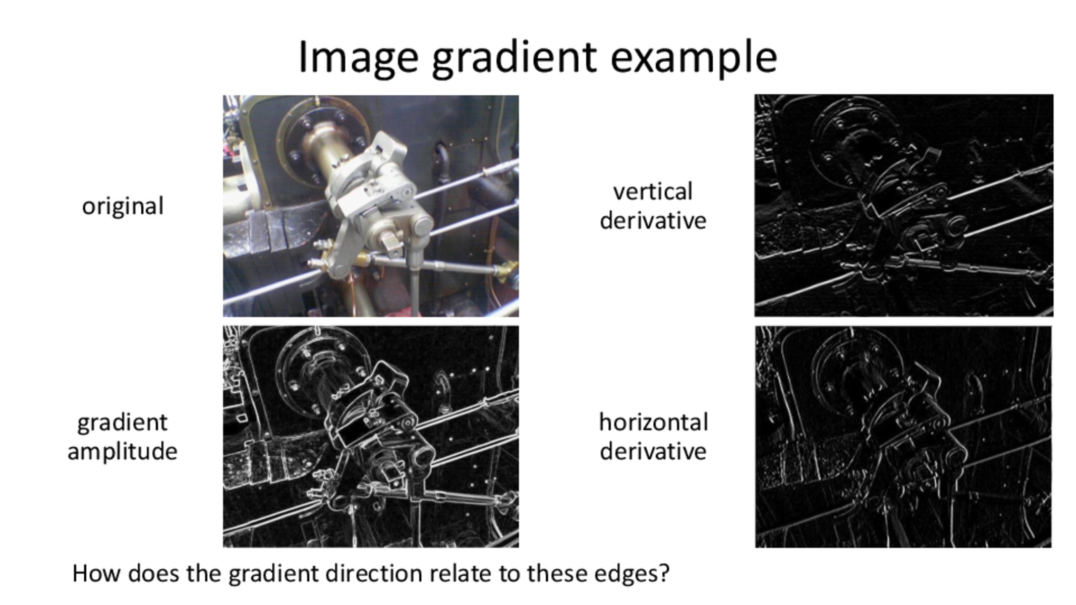
In the gradient amplitude image, I presume we have simply created an image based on the gradient amplitude function on the previous slide.
How does this compare to simply overlaying the vertical and horizontal derivative images? Also, to clarify, the vertical and horizontal derivative images are just the product of convolving the sobel filters with the image as described in step 2 of the previous slide, right? And also thus equivalent to the edge detection slides from before?
motoole2
Yes, the gradient amplitude image is the result of computing the following per pixel: $\sqrt{I_x^2 + I_y^2}$, where $I_x$ and $I_y$ represent the x- and y- gradients. If you think of the gradient as an arrow pointing in the direction of the largest change in intensity $[I_x,I_y]$, the amplitude represents the length of this arrow. Note that, when computing the gradient amplitude image of a line, the result would be invariant to the orientation of said line.
How does this compare to overlaying the two derivative images, i.e., $I_x + I_y$? First, you would need to take into consideration the fact that the derivative images contain negative values, perhaps by summing up the absolute value of these derivative images $abs(I_x) + abs(I_y)$ instead. This produces something that looks similar to the amplitude image in the slide, except that the result would no longer be invariant to orientation of a line.
(And yes, the vertical and horizontal derivative images are the result of convolving the Sobel filters with the image.)
In the gradient amplitude image, I presume we have simply created an image based on the gradient amplitude function on the previous slide.
How does this compare to simply overlaying the vertical and horizontal derivative images? Also, to clarify, the vertical and horizontal derivative images are just the product of convolving the sobel filters with the image as described in step 2 of the previous slide, right? And also thus equivalent to the edge detection slides from before?
Yes, the gradient amplitude image is the result of computing the following per pixel: $\sqrt{I_x^2 + I_y^2}$, where $I_x$ and $I_y$ represent the x- and y- gradients. If you think of the gradient as an arrow pointing in the direction of the largest change in intensity $[I_x,I_y]$, the amplitude represents the length of this arrow. Note that, when computing the gradient amplitude image of a line, the result would be invariant to the orientation of said line.
How does this compare to overlaying the two derivative images, i.e., $I_x + I_y$? First, you would need to take into consideration the fact that the derivative images contain negative values, perhaps by summing up the absolute value of these derivative images $abs(I_x) + abs(I_y)$ instead. This produces something that looks similar to the amplitude image in the slide, except that the result would no longer be invariant to orientation of a line.
(And yes, the vertical and horizontal derivative images are the result of convolving the Sobel filters with the image.)